DC Network Theorem, Basic Electrical Engineering, Btech first year

DC Network Theorems

• Some Basic Terms & Definitions

  Electric Circuit : It is a closed path composed of active and passive elements in which electric current flows.
  
  Active Element : It is the element in the circuit which provides energy to the circuit. Example- battery
  
  Passive Element : It is the element in the circuit which receives energy and convert it to heat or stores it. Example- capacitor, resistor
  
  Active Network : A network which contains one or more than one sources of e.m.f.
  
  Passive Network : A network which contains no source of e.m.f.
  
  Linear Circuit : A Linear circuit is one whose parameters are constant i.e. they do not change with voltage or current.
  
  Non-Linear Circuit : It is that circuit whose parameters change with voltage or current.
  
  Bilateral Elements : Elements which allow flow of current in both the directions.
  
  Unilateral Elements : Elements which allow flow of current in only one direction.
  
  Node : It is a point in a circuit where two or more elements are connected.
  
  Junction : A point where three or more than three branches combine or the point where current divides.
  
  Branch : is a part of a network which lies in between two junctions.
  
  Loop : It is a closed path in a circuit in which no element or node is encountered more than once.
  
  Mesh : It is a loop that contains no other loop within it.
  
  Ohm's Law : The potential difference across any two points of conductor will be directly proportional to current flowing through it.
  \[ V \propto I \] \[ \boxed{V = IR} \] Kirchoff's Laws:
  1) Kirchoff's Voltage Law : (Based on Law of Conservation of Energy) In any closed circuit or mesh, algebraic sum of all EMFs and voltage drops is 0.
  \[ \sum EMFs + \sum IR = 0 \] Direction of Current
  (a) If current is flowing from lower to higher potential (\(-ve\) to \(+ve\)) \(\longrightarrow\) Rise in potential \(\Rightarrow\) current is positive
  (b) If current is flowing from higher to lower potential (\(+ve\) to \(-ve\)) \(\longrightarrow\) Drop in potential \(\Rightarrow\) current is negative
  
  2) Kirchoff's Current Law : (Based on Law of Conservation of Charge) The algebraic sum of all the currents meeting at a point or a junction is 0. \[ \sum I = 0 \]

• Star-Delta Transformation

  Derivation :

  Delta \(\longrightarrow\) Star :

  

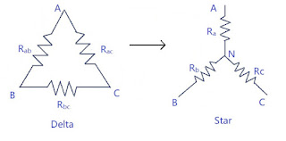
  Between node \(A\) and \(B\) : \[ R_{ab} || (R_{ac} + R_{bc}) \] \[ \frac{ R_{ab} \times (R_{ac} + R_{bc})}{R_{ab} + R_{ac} + R_{bc}} = R_a + R_b \hspace{20pt} \longrightarrow (1) \] Between node \(B\) and \(C\) : \[ R_{bc} || (R_{ab} + R_{ac}) \] \[ \frac{ R_{bc} \times (R_{ab} + R_{bc})}{R_{ab} + R_{ac} + R_{bc}} = R_b + R_c \hspace{20pt} \longrightarrow (2) \] Between node \(A\) and \(C\) : \[ R_{ac} || (R_{ab} + R_{bc}) \] \[ \frac{ R_{ac} \times (R_{ab} + R_{bc})}{R_{ab} + R_{ac} + R_{bc}} = R_a + R_c \hspace{20pt} \longrightarrow (3) \] Adding equations 1, 2, 3 \[ 2(R_a + R_b + R_c) = 2\frac{R_{ab}R_{bc} + R_{bc}R_{ac} + R_{ac}R_{ab}}{R_{ab} + R_{ac} + R_{bc}} \] \[ \boxed{ R_a + R_b + R_c = \frac{R_{ab}R_{bc} + R_{bc}R_{ac} + R_{ac}R_{ab}}{R_{ab} + R_{ac} + R_{bc}} } \hspace{10pt} \longrightarrow (4) \] Equation (4) - (1) \[ R_c = \frac{ R_{ab}R_{bc} + R_{bc}{ac} + R_{ac}R_{ab} }{ R_{ab} + R_{ac} + R_{bc} } - \frac{ R_{ab}R_{ac} + R_{ab}R_{bc} }{ R_{ab} + R_{bc} + R_{ac} } \] \[ \boxed{ R_c = \frac{ R_{bc}R_{ac} }{ R_{ab} + R_{bc} + R_{ac} } } \hspace{10pt} \longrightarrow (5) \] \[ \boxed{ R_a = \frac{ R_{ab}R_{ac} }{ R_{ab} + R_{bc} + R_{ac} } } \longrightarrow (6) \] \[ \boxed{ R_b = \frac{ R_{bc}R_{ab} }{ R_{ab} + R_{bc} + R_{ac} } } \longrightarrow (7) \]

  Star \(\longrightarrow\) Delta :

  

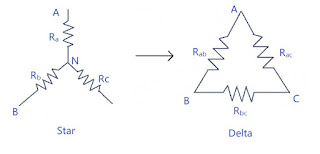
  Multiplying (7) and (6) \[ R_a\times R_b = \frac{ R_{ab}^2\times R_{ac}\times R_{bc} }{ (R_{ab} + R_{ac} + R_{bc})^2 } \hspace{10pt} \longrightarrow (8) \] Multiplying (6) and (5) \[ R_a\times R_c = \frac{ R_{ac}^2\times R_{ab}\times R_{bc} }{ (R_{ab} + R_{ac} + R_{bc})^2 } \hspace{10pt} \longrightarrow (9) \] Multiplying (5) and (7) \[ R_b\times R_c = \frac{ R_{bc}^2\times R_{ac}\times R_{ab} }{ (R_{ab} + R_{ac} + R_{bc})^2 } \hspace{10pt} \longrightarrow (10) \] Adding (8) (9) and (10) \[ R_aR_b + R_bR_c + R_cR_a = \frac{ R_{ab}^2R_{ac}R_{bc} + R_{ac}^2R_{bc}R_{ab} + R_{bc}^2R_{ab}R_{ac} }{ R_{bc}^2\times R_{ac}\times R_{ab} } \] \[ R_aR_b + R_bR_c + R_cR_a = \frac{ R_{ab}R_{ac}R_{bc}\cancel{(R_{ab} + R_{ac} + R_{bc})} }{ (R_{ab} + R_{ac} + R_{bc})^\cancel{2} } \] \[ R_aR_b + R_bR_c + R_cR_a = R_a\times R_{bc} \] \[ \boxed{ R_{bc} = \frac{ R_aR_b + R_bR_c + R_cR_a }{R_a} } \hspace{10pt} \longrightarrow (11) \] Similarly \[ R_aR_b + R_bR_c + R_cR_a = R_{ab}\times R_c \] \[ \boxed{ R_{ab} = \frac{ R_aR_b + R_bR_c + R_cR_a }{R_c} } \hspace{10pt} \longrightarrow (12) \] \[ R_aR_b + R_bR_c + R_cR_a = R_{ac}\times R_b \] \[ \boxed{ R_{ac} = \frac{ R_aR_b + R_bR_c + R_cR_a }{R_b} } \hspace{10pt} \longrightarrow (13) \]

• Mesh Analysis

  An important step in Mesh Analysis is identifying meshes so here is a quick example:
  
  

  

  In this figure, \(ABEF \rightarrow\) a Mesh \(\rightarrow\) also a Loop
  \(BCDE \rightarrow\) a Mesh \(\rightarrow\) also Loop
  \(ACDF \rightarrow \) not a Mesh \(\rightarrow\) a Loop

  Sample Problem 1 :

  Calculate current in the branch of \(2\Omega\) resistance for the given circuit using Mesh Analysis

  

  Solution:

  

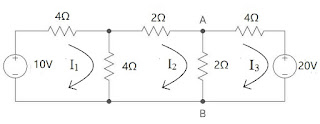
  First we will identify meshes in the given circuit. There are three meshes in the circuit. In each mesh, current is flowing in clockwise direction.
  Second apply KVL in mesh (1) : \[+10 - 4I_1 - 4(I_1 - I_2) = 0 \] \[ \boxed{-8I_1 + 4I_2 + 0I_3 = -10} \hspace{20pt} \longrightarrow (1) \] Applying KVL in mesh (2) : \[ -4(I_2 - I_1) - 2I_2 - 2(I_2 - I_3) = 0 \] \[ \boxed{4I_1 - 8I_2 + 2I_3 = 0} \hspace{20pt} \longrightarrow (2) \] Applying KVL in mesh (3) : \[ -2(I_3 - I_2) - 4I_3 - 20 = 0 \] \[ \boxed{0I_1 + 2I_2 - 6I_3 = 20} \hspace{20pt} \longrightarrow (3) \] Now, \( AI = B, \text{ where I is current matrix } \) \[ \begin{bmatrix} -8 &4 &0\\ 4 &-8 &2\\ 0 &2 &-6 \end{bmatrix} \begin{bmatrix} I_1\\ I_2\\ I_3 \end{bmatrix} = \begin{bmatrix} -10\\ 0\\ 20 \end{bmatrix} \] Using Cramer's rule : \[ \begin{vmatrix} A \end{vmatrix} = -8(48 - 4) - 4(-24) = -256 \] \[ \text{For } I_1, \hspace{20pt} A_1 = \begin{bmatrix} -10 &4 &0\\ 0 &-8 &2\\ 20 &2 &-6 \end{bmatrix} \] \[ \begin{vmatrix} A_1 \end{vmatrix} = -10(-4) - 4(-40) = 200 \] \[ I_1 = \frac{\begin{vmatrix} A_1 \end{vmatrix}}{\begin{vmatrix} A \end{vmatrix}} = \frac{200}{-256} \] \[ \Rightarrow \boxed{I_1 = -0.781 A} \] \[ \text{For } I_2, \hspace{20pt} A_2 = \begin{bmatrix} -8 &-10 &0\\ 4 &0 &2\\ 0 &20 &-6 \end{bmatrix} \] \[ \begin{vmatrix} A_2 \end{vmatrix} = -8(-40) + 10(-24) = 80 \] \[ I_2 = \frac{\begin{vmatrix} A_2 \end{vmatrix}}{\begin{vmatrix} A \end{vmatrix}} = \frac{80}{-256} \] \[ \Rightarrow \boxed{I_2 = -0.312 A} \] \[ \text{For } I_3, \hspace{20pt} A_3 = \begin{bmatrix} -8 &4 &-10\\ 4 &-8 &0\\ 0 &2 &20 \end{bmatrix} \] \[ \begin{vmatrix} A_3 \end{vmatrix} = -8(-160) - 4(80) -10(8) = 880 \] \[ I_3 = \frac{\begin{vmatrix} A_3 \end{vmatrix}}{\begin{vmatrix} A \end{vmatrix}} = \frac{880}{-256} \] \[ \Rightarrow \boxed{I_3 = -3.437 A} \] Now current in the required \(2\Omega\) branch will be equal to \( I_2 - I_3 \) \[ I = I_2 - I_3 = -0.312 + 3.437 \] \[ \boxed{I = 3.125 A} \]

  Sample Problem 2 :

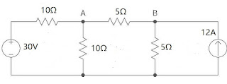
  Find the current in \(A-B\) using mesh analysis

  

  Solution:

  

  There are 3 meshes in the circuit
  Applying KVL in mesh 1 : \[ 30 - 10I_1 - 10(I_1 - I_2) = 0 \] \[ -20I_1 + 10I_2 = -30 \] \[ \boxed{-2I_1 + I_2 = -3} \hspace{20pt} \Rightarrow (1) \] Applying KVL in mesh 2 : \[ -10(I_2 - I_1) - 5I_2 - 5(I_2 - I_3) = 0 \] \[ 10I_1 - 20I_2 + 5I_3 = 0 \] \[ \boxed{2I_1 - 4I_2 + I_3 = 0} \hspace{20pt} \Rightarrow (2) \] Applying KVL in mesh 3, since there is only a current source : \[ I_3 = -12 A \] So putting the value in equation (2) : \[ \boxed{2I_1 + 4I_2 = 12} \hspace{20pt} \Rightarrow (3) \] Now, \( AI = B, \text{ where I is current matrix } \) \[ \begin{bmatrix} -2 &1 \\ 2 &-4 \end{bmatrix} \begin{bmatrix} I_1\\ I_2\\ \end{bmatrix} = \begin{bmatrix} -3\\ 12 \end{bmatrix} \] Using Cramer's rule : \[ \begin{vmatrix} A \end{vmatrix} = 8 - 2 = 6 \] \[ \text{For } I_1, \hspace{20pt} A_1 = \begin{bmatrix} -3 &1\\ 12 &-4 \end{bmatrix} \] \[ \begin{vmatrix} A_1 \end{vmatrix} = 12 - 12 = 0 \] \[ I_1 = \frac{\begin{vmatrix} A_1 \end{vmatrix}}{\begin{vmatrix} A \end{vmatrix}} = \frac{0}{6} \] \[ \Rightarrow \boxed{I_1 = 0 A} \] \[ \text{For } I_2, \hspace{20pt} A_2 = \begin{bmatrix} -2 &-3\\ 2 &12 \end{bmatrix} \] \[ \begin{vmatrix} A_2 \end{vmatrix} = -24 + 6 = -18 \] \[ I_2 = \frac{\begin{vmatrix} A_2 \end{vmatrix}}{\begin{vmatrix} A \end{vmatrix}} = \frac{-18}{6} \] \[ \Rightarrow \boxed{I_2 = -3 A} \] \[ \boxed{I_{AB} = I_2 = -3 A} \]

• Nodal Analysis

  Steps for solving numericals using Nodal Analysis :

  1) Identify the principal nodes or junctions in the network
  2) Pick a reference junction in the circuit with value \(V_0 = 0V\)
  3) Assign a junction potential on each junction with respect to the reference junction
  4) Assuming all the currents in outgoing (or incoming) direction from each junction, form KCL equations
  5) Solve the equations and calculate value of the junction potentials
  6) Using individual junction potentials find the value of required quantity

  
  

  Sample Problem:

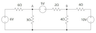
  Find the current in \(3\Omega\) resistor using Nodal Analysis

  

  Solution:

  

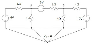
  Applying KCL at junction A : \[ I_1 + I_2 + I_3 = 0 \] \[ \frac{V_A - V_0 - 6}{6} + \frac{V_A - V_0}{3} + \frac{V_A - V_B + 5}{2} = 0 \] \[ \frac{V_A - V_0 - 6 + 2V_A - 2V_0 + 3V_A - 3V_B + 15}{6} = 0 \] \[ 6V_A - 3V_B = -9 \] \[ \boxed{2V_A - V_B = -3} \hspace{20pt} \longrightarrow (1) \] Applying KCL at junction B : \[ I_1 + I_2 + I_3 = 0 \] \[ \frac{V_B - V_A - 5}{2} + \frac{V_B - V_0}{4} + \frac{V_B - V_0 - 10}{4} = 0 \] \[ \frac{2V_B - 2V_A - 10 + V_B + V_B - 10}{4} = 0 \] \[ -2V_A + 4V_B = 20 \] \[ \boxed{-V_A + 2V_B = 10} \hspace{20pt} \longrightarrow (2) \] Now, \( AV = B, \text{ where I is voltage matrix } \) \[ \begin{bmatrix} 2 &-1 \\ -1 &2 \end{bmatrix} \begin{bmatrix} V_A\\ V_B\\ \end{bmatrix} = \begin{bmatrix} -3\\ 10 \end{bmatrix} \] Using Cramer's rule : \[ \begin{vmatrix} A \end{vmatrix} = 4 - 1 = 3 \] \[ \text{For } V_A, \hspace{20pt} A_1 = \begin{bmatrix} -3 &-1\\ 10 &2 \end{bmatrix} \] \[ \begin{vmatrix} A_1 \end{vmatrix} = -6 + 10 = 4 \] \[ V_A = \frac{\begin{vmatrix} A_1 \end{vmatrix}}{\begin{vmatrix} A \end{vmatrix}} = \frac{4}{3} = 1.33 V \] \[ \text{For } V_B, \hspace{20pt} A_2 = \begin{bmatrix} 2 &-3\\ -1 &10 \end{bmatrix} \] \[ \begin{vmatrix} A_2 \end{vmatrix} = 20 - 3 = 17 \] \[ V_B = \frac{\begin{vmatrix} A_2 \end{vmatrix}}{\begin{vmatrix} A \end{vmatrix}} = \frac{17}{4} = 4.25 V \] \[ I_{3\Omega} = I_2 = \frac{V_A - V_0}{3} \] \[ \boxed{I_{3\Omega} = 0.443 A} \]

• Thevenin's Theorem

  Thevenin's Theorem : It states that any linear bilateral network can be simplified into a Thevenin's equivalent circuit having Thevenin's open circuit voltage \(V_{Th}\) in series with the Thevenin's equivalent resistance \(R_{Th}\) along with load resistance \(R_{L}\)

  

  \[ \boxed{I_L = \frac{V_{Th}}{R_L + R_{Th}} } \]

  Steps for solving :

  1) Identify the load resistance \(R_L\)
  2) Remove the load resistance and calculate the open circuit voltage across the two open ends \(\longrightarrow V_{Th}\)
  3) Again remove \(R_L\) and replace all the active sources by their internal resistance: \[\rightarrow \text{for voltage source: Internal resistance } = 0 \Rightarrow short-circuit \] \[\rightarrow \text{for current source: Internal resistance } = \infty \Rightarrow open-circuit \] 4) Calculate equivalent resistance across the open ends \(\rightarrow R_{Th}\)
  5) Draw the Thevenin Equivalent circuit
  6) Calculate load current \(I_L\) by using \[ \boxed{I_L = \frac{V_{Th}}{R_L + R_{Th}} } \]

  
  

  Sample Problem

  Find the current through \(1\Omega\) resistor in given circuit using Thevenin's Theorem :

  

  Solution :

  Step 1: Load Resistance, \(R_L = 1\Omega \)
  Step 2: Removing \(R_L\) to find \(V_{Th} \)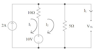

  

  Applying KVL in mesh 1 \[ \boxed{I_1 = 2 A} \] Applying KVL in mesh 2 \[ 10 - 10(I_2 - I_1) - 5I_2 = 0 \] \[ 10 - 10(I_2 - 2) - 5I_2 = 0 \] \[ \boxed{I_2 = 2 A} \] In mesh 3, for \(5\Omega\) resistor, \(V = IR = 2\times5 = 10 V\)
  Applying KVL, \[ -V_{Th} + 10 = 0 \Rightarrow \boxed{V_{Th} = 10 V } \] Step 3: Removing \(R_L\) and replacing all the acive sources by their internal resistance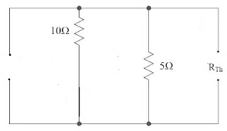

  

  Step 4: Equivalent Resistance across the open ends, \[ R_{Th} = 10 || 5 = \frac{10\times5}{10+5} = \frac{50}{13} = 3.33 \Omega \] Step 5: Thevenin's Equivalent circuit,

  

  Sstep 6: Calculate Load Current, \[ I_L = \frac{V_{Th}}{R_{Th} + R_L} = \frac{10}{4.33} \] \[ \boxed{I_L = 2.31 A} \]

• Norton's Theorem

  Norton's Theorem : Any linear bilateral network irrespective of its complexity can be reduced to Norton's Equivalent circuit having a Norton's short circuit current \(I_N\) in parallel with Norton's equivalent resistance \(R_N\) in parallel with load resistance \(R_L\)

  

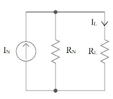
  \[ \boxed{I_L = \frac{I_NR_N}{R_N + R_L} } \]

  Steps for solving :

  1) Identify the load resistance \(R_L\)
  2) Replace \(R_L\) with short circuited branch
  3) The current flowing through this short circuit branch will be the Norton's current \(I_N\)
  4) Remove \(R_L\) and replace all the active sources by their internal resistance
  5) The equivalent resistance across the two open ends will be the Norton's resistance \(R_N\)
  6) Draw Norton's equivalent circuit
  7) Calculate \(I_N\) using identity : \[ \boxed{I_N = \frac{I_NR_N}{R_N + R_L} } \]

  Sample Problem :

  Find the current \(I'\) in the given circuit using Norton's Theorem :

  

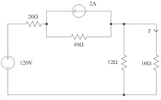
  Solution:

  Step 1: Load Resistance, \(R_L = 10\Omega\)
  Step 2: Replacing \(R_L\) with short circuit branch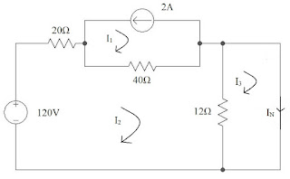

  

  Step 3: Finding \(I_N\),
  Applying KVL in mesh 1, \[ \boxed{I_1 = -2 A}\]
  Applying KVL in mesh 2, \[ 120 - 20I_2 - 40(I_2 - I_1) -12(I_2 - I_3) \] \[ 10I_1 - 18I_2 + 3I_3 = -30 \] \[ \boxed{-18I_2 + 3I_3 = -10} \hspace{20pt} \longrightarrow (1) \] Applying KVL in mesh 3, \[ -12(I_3 - I_2) = 0 \] \[ \boxed{I_2 = I_3} \] In equation (1) \[ -18I_2 + 3I_2 = -10 \] \[ I_2 = 0.666 A \] \[ \boxed{I_N = I_3 = 0.666 A} \] Step 4: Removing \(R_L\) and replacing all active sources by their internal resistances

  

  Step 5: Calculating Equivalent resistance, \[ R_N = (20 + 40)||12 = 60||12 = 10\Omega \] Step 6: Norton's equivalent circuit,

  

  Step 7: Calculate \(I_L\), \[ I_L = \frac{I_NR_N}{R_N + R_L} = \frac{0.666\times10}{10 + 10} \] \[ \boxed{I_L = I' = 0.333 A} \]

• Superposition Theorem

  Superposition Theorem : In any linear bilateral multisource network the current or voltage across any branch can be calculated by taking the algebraic sum of values calculated by taking one source at a time and replacing all the remaining sources by their internal resistances.

  Steps for solving:

  1) Identify the active sources and the quantity to be calculated
  2) Consider any one active source and replace the remaining sources by their internal resistances
  3) Calculate the required electrical quantity for that particular source
  4) Repeat step 2 and 3 for remaining sources
  5) Algebraic sum of all these individual values will be the final value of required electrical quantity for all the sources working together

  
  

  Sample Problem :

  For given circuit calculate I' using Superposition Theorem:

  

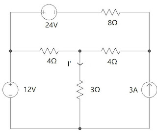
  Solution :

  Step 1: There are two volatage sources and one current source
  Step 2: Considering \(12 V\) source and replacing the remaining sources with their internal resistances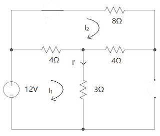

  

  Applying KVL in mesh 1, \[ 12V - 4(I_1 - I_2) - 3I_1 = 0 \] \[ -7I_1 + 4I_2 = -12 \hspace{20pt} \longrightarrow (1) \] Applying KVL in mesh 2, \[ -8I_2 - 4I_2 - 4(I_2 - I_1) = 0 \] \[ \boxed{I_1 = 4I_2} \] Putting \(I_1\) in equation (1) \[ -28I_2 + 4I_2 = -12 \] \[ \boxed{I_2 = 0.5 A} \] \[ \boxed{I_1 = 2 A} \] \[ \boxed{I_{12v} = I_1 = 2A} \]
  Taking \(24 V\) source and replacing the remaining sources with their internal resistances

  

  Applying KVL in mesh 1, \[ -3I_1 - 4(I_1 - I_2) = 0 \] \[ I_2 = \frac{7I_1}{4} \] Applying KVL in mesh 2, \[ -24 - 8I_2 - 4I_2 - 4(I_2 - I_1) = 0 \] \[ -16I_2 + 4I_1 = 24 \] \[ -28I_1 + 4I_1 = 24 \] \[ \boxed{I_! = -1 A} \] \[ I_2 = \frac{-7}{4} \] \[ \boxed{I_2 = -1.75 A} \] \[ \boxed{I_{24V} = I_1 = -1A} \]
  Taking \(3 A\) source and replacing the remaining sources with their internal resistances

  

  Applying KVL in mesh 2, \[ \boxed{I_2 = -3A} \] Applying KVL in mesh 1, \[ -4(I_1 - I_3) - 3(I_1 - I_2) = 0 \] \[ \boxed{-7I_1 + 4I_3 = 9} \hspace{20pt} \longrightarrow (1) \] Applying KVL in mesh 3, \[ -8I_3 - 4(I_3 - I_2) - 4(I_3 - I_1) = 0 \] \[ 4I_1 - 16I_3 = 12 \] \[ \boxed{I_1 - 4I_3 = 3} \hspace{20pt} \longrightarrow (2) \] \[ \begin{bmatrix} -7 &4\\ 1 &-4 \end{bmatrix} \begin{bmatrix} I_1\\ I_3 \end{bmatrix} \] \[ \begin{vmatrix} A \end{vmatrix} = 28 - 4 =24 \] \[ A_1 = \begin{bmatrix} 9 &4\\ 3 &-4 \end{bmatrix} \] \[ \begin{vmatrix} A_1 \end{vmatrix} = -36 - 12 = -48 \] \[ I_1 = \frac{-48}{24} = -2A \] \[ A_2 = \begin{bmatrix} -7 &9\\ 1 &3 \end{bmatrix} \] \[ \begin{vmatrix} A_1 \end{vmatrix} = -21 -9 = -30 \] \[ I_3 = \frac{-30}{24} = -1.25 A \] \[ I_2 = -3 A \] \[ I_{3A} = I_1 - I_2 \] \[ \boxed{I_{3A} = 1A }\] Total Current, \( I_T = I_{12V} + I_{24V} + I_{3A} \) \[ \boxed{I_T = 2A }\]

• Maximum Power Transfer Theorem

  Maximum Power Transfer Theorem : The condition for maximum power flow through load resistor \(R_L\) can be acheived when the load resistor equals the Thevenin's equivalent resistance of the circuit.

  

  Power through \(R_L\) \[ P = I_l^2R_L \] \[ I_L = \frac{V_{Th}}{R_{Th} + R_{L} } \] \[ P = (\frac{V_{Th}}{R_{Th} + R_L})^2R_L \] Differentiating above equation with respect to \(R_L\) and equating it to 0 \[ \frac{dP}{dR_L} = V_{Th}^2[ \frac{(R_{Th} + R_L)^2 - 2R_L(R_{Th} + R_L)}{(R_{Th} + R_L)^4} ] \] \[ R_{Th}^2 - R_L^2 = 0\] \[ \boxed{R_{Th} = R_L }\] This is the condition for maximum power flow \[ P = ( \frac{V_{Th}}{R_{Th} + R_L} )^2R_L \] \[ = \frac{V_{Th}^2}{4R_{Th}^2} \times R_{Th} \] \[ \boxed{P_{max} = \frac{V_{Th}^2}{4R_{Th}}} \]

  
  

  Sample Problem:

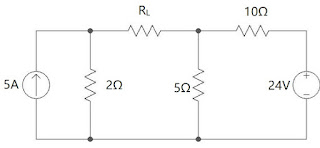
  In the given network find the value of \(R_L\) which will absorb the maximum power from the source. Also find the maximum power.

  

  Solution

  For \(V_{Th}\), removing \(R_L\)

  

  Applying KVL in mesh 1: \[ \boxed{I_1 = 5 A} \] Applying KVL in mesh 2: \[ -5I_2 - 10I_2 = 24V \] \[ \boxed{I_2 = -1.6 A} \] \[ -V_{Th} - 8 + 10 = 0 \] \[ \boxed{V_{Th} = 2 V} \] Removing \(R_L\) and replacing all active sources with their internal resistances

  

  \[ R_{Th} = 2 + 5||10 \] \[ R_{Th} = 2 + \frac{50}{15} \] \[ \boxed{R_{Th} = 5.33 \Omega } \] For maximum power flow, \( R_L = R_{Th} = 5.33 \Omega \) \[ P_{max} = \frac{ V_{Th}^2 }{4R_{Th}} \] \[ P_{max} = \frac{4}{4\times5.33} \] \[ \boxed{P_{max} = 0.187 W} \]

Triple Integration Engineering Maths, Btech first year

Triple Integration

In Triple Integration, we integrate w.r.t. 3 variables. Here we are going to study two types:
Type-1 : Constant limits
Type-2 : Variable limits

Type-1 : Constant limits

\[ \int_0^1 \int_0^2 \int_0^3 xy^2z^3dxdydz \] The rule is same as Double Integration \[ \text{Inner Variable} \longrightarrow \text{Inner Limit} \] \[ \text{Outer Variable} \longrightarrow \text{Outer Limit} \] So here \(x\) will have limits 0 to 3, \(y\) will have limits 0 to 2 and \(z\) will have limits 0 to 1. Let's integrate: \[ = \int^1_0 \int^2_0 \left[\frac{x^2}{2} \right]^3_0y^2z^3dydz \] \[ = \frac{9}{2} \int^1_0 \int^2_0 y^2z^3dydz \] \[ = \frac{9}{2} \int_0^1 \left[\frac{y^3}{3} \right]^2_0 z^3dz \] \[ = \frac{9}{2}\times \frac{8}{3} \int^1_0 z^3dz \] \[ = 12 \left[\frac{z^4}{4} \right]_0^1 \] \[ = \boxed{3} \]

Type-2 : Variable Limits

\[ \int^a_0 \int^x_0 \int^{x+y}_0 e^{x+y+z}dxdydz \] Like in Double Integration, here \(x + y\) is in terms of \(z\) so it will be limits of \(z\) and the limit \(x\) belongs to \(y\). Let's integrate: \[ = \int^a_0 \int^x_0\left[e^{x+y+z} \right]^{x+y}_0dxdy \] \[ = \int^a_0 \int^x_0\left[e^{x+y+(x+y)} - e^{x+y+0} \right]dxdy \] \[ = \int^a_0 \int^x_0\left[e^{2x+2y} - e^{x+y} \right]dxdy \] \[ = \int^a_0 \left[\frac{e^{2x+2y}}{2} - \frac{e^{x+y}}{1} \right]^x_0 dx \] \[ = \int^a_0 \left[\left(\frac{e^{2x+2x}}{2} - \frac{e^{x+x}}{1}\right) - \left(\frac{e^{2x+0}}{2} - \frac{e^{x+0}}{1} \right) \right]dx \] \[ = \int^a_0 \left[\left(\frac{e^{4x}}{2} - e^{2x}\right) - \left(\frac{e^{2x}}{2} - e^{x} \right) \right]dx \] \[ = \int^a_0 \left[\frac{e^{4x}}{2} - \frac{3e^{2x}}{2} + e^x \right]dx \] \[ = \left[\frac{e^{4x}}{8} - \frac{3e^{2x}}{4} + e^x \right]^a_0 \] \[ = \frac{e^{4a}}{8} - \frac{3e^{2a}}{4} + e^a - \left(\frac{1}{8} - \frac{3}{4} + 1 \right) \] \[ = \frac{e^{4a} - 6e^{2a} + 8e^a + 3}{8} \]

Basic Formula for Integration Engineering Maths, Btech first year

Basic Formulas for Integration

Below are some basic formulas that you may want to revise: \[ 1)\hspace{5pt} \int x^ndx = \frac{x^{n+1}}{n+1} + C, n \neq 1 \] \[ 2)\hspace{5pt} \int \cos{x}dx = \sin{x} + C \] \[ 3)\hspace{5pt} \int \sin{x}dx = -\cos{x} + C \] \[ 4)\hspace{5pt} \int \sec^2{x}dx = \tan{x} + C \] \[ 5)\hspace{5pt} \int cosec^2xdx = -\cot{x} + C \] \[ 6)\hspace{5pt} \int \sec{x}\tan{x}dx = \sec{x} + C \] \[ 7)\hspace{5pt} \int cosecxcotxdx = -cosecx + C \] \[ 8)\hspace{5pt} \int \frac{dx}{\sqrt{1-x^2}} = \sin^{-1}{x} + C \] \[ 9)\hspace{5pt} \int \frac{dx}{\sqrt{1-x^2}} = -\cos^{-1}{x} + C \] \[ 10)\hspace{5pt} \int \frac{dx}{1+x^2} = tan^{-1}x + C \] \[ 11)\hspace{5pt} \int (3x+5)^{10}dx = \frac{(3x+5)^{11}}{(11)(3)} \]

Integration by parts

\[ \int uvdx \neq \int udx.\int vdx \] \[ \int uvdx = u \int vdx - \int \left[\frac{d}{dx}(u) \int vdx \right]dx \] Priority for types of different types of functions is given by ILATE:
I \(\longrightarrow \) Inverse Trigonometric function
L \(\longrightarrow \) Logarithmic function
A \(\longrightarrow \) Algebraic function
T \(\longrightarrow \) Trigonometric function
E \(\longrightarrow \) Exponential function

Example : \[ \int xe^xdx \] In this problem, our first function will be \(x\) and second function will be \(e^x\) \[ = x \int e^xdx - \int \left[\frac{d}{dx}(x) \int e^xdx \right]dx \] \[ = xe^x - \int e^x dx \] \[ = xe^x - e^x + C \]

Double Integration Engineering Maths, Btech first year

Double Integration

Before we jump into Double Integration, if you need to revise some basic concepts of Integration Click Here.

In normal Integration we would perform integration w.r.t. only one variable; in Double Integration we will perform integration w.r.t. two variables.

Here we are going to study three types of Double Integration:
Type 1 : With constant limits
Type 2 : With variable limits
Type 3 : No limits \(\longrightarrow\) we would have to find out from the question

Type-1 : With constant limits :

\[ \int_0^4\int_0^{10} xydxdy \] Here the confusion is- which variable has which limits, so below is the rule: \[ \text{Inner Variable} \longrightarrow \text{Inner Limit} \] \[ \text{Outer Variable} \longrightarrow \text{Outer Limit} \] In this problem \(x\) has limits 0 to 10, \(\hspace{5pt} y\) has limits 0 to 4.
And there is no rule for which variable has to be integrated first so you can either first integrate \(x\) and then \(y\) or vice-versa. Let's integrate the above problem in both orders:

1) First \(x\), then \(y\)

\[ \int^4_0 \left[\frac{x^2}{2} \right]^{10}_0ydy = 50\int^4_0ydy \] \[ = 50\left[\frac{y^2}{2} \right]^4_0 = 50 \times 8 = 400 \]

2) First \(y\), then \(x\) :

\[ \int^{10}_0 x\left[\frac{y^2}{2} \right]^{4}_0dx = 8\int^{10}_0xdx \] \[ = 8\left[\frac{x^2}{2} \right]^4_0 = 8 \times 50 = 400 \] As you can see, answers in both the cases are same.

Type-2 : With variable limits

\[ \int^1_0 \int^x_{x^2} xydxdy \] Here the rule that you used in first type is not applicable. In this type, one limit consists of \(x\) variable, so the question is: to which variable does it belong? The answer is simple, consider this: does \(x = x \) make any sense to you? No. Does \(y = x \) make sense to you? Yes. Why? Because in first equation \(x\) was written in terms of \(x\) which just doesn't make any sense and in the second equation, \(x\) was written in terms of \(y\) which is obvious. So from this you can conclude that if the limit consists of \(x\) variable, then it must belong to \(y\) and if the limit consists of \(y\) variable, then it must belong to \(x\).
Also here the order of integration matters: the one with variable limits will be integrated first. So let's solve the above problem:

\[ \int_0^1 \left[\frac{y^2}{2} \right]^x_{x^2} xdx \] \[ = \int^1_0 \left[\frac{x^2}{2} - \frac{x^4}{2} \right]xdx \] \[ = \frac{1}{2}\int^1_0 \left(x^3 - x^5 \right)dx \] \[ = \frac{1}{2}\left[\frac{x^4}{4} - \frac{x^6}{6} \right]^1_0 \] \[ = \frac{1}{2}\left(\frac{1}{4} - \frac{1}{6} \right) = \frac{1}{24} \]

Type 3 : No limit

In this type of problems, we won't be given limits, instead we will be given equations of lines or curves which we will use to determine the region in cartesian plane over which we will integrate the given integral. Let's see an example :

Sample Problem 1

Evaluate \(\hspace{5pt} \iint xydxdy \hspace{5pt}\) over positive quadrant of the circle \( x^2 + y^2 = a^2 \)

Solution

In these kind of problems, we follow the following steps:
1) Trace the curve using the equations of curves given in the question
2) Identify the region over which we will integrate
3) Find the limits
4) Integrate
Step-1 : Trace the curve \[ x^2 + y^2 = a^2 \] It is a circle of radius \(a\) units and center (0,0).

Step-2 : identify the region
Here it is given the positive quadrant so,

Step-3 : Find the limits
Now comes the main part. There are two ways to find limits, Horizontal Strip or Vertical Strip. Now consider this, integration is all about finding area, so how do you find area of such region? Simple, take a strip, and drag it to cover the whole region. Here you have two ways: Horizontal Strip or Vertical Strip.

If you take a horizontal strip, it will be parallel to the x-axis and vertical strip will be parallel to y-axis. The both ends of the strip will be the limits i.e. the equation of the curves they are touching: if horizontal strip, then limits will belong to \(x\), if vertical strip, then the limits will belong to \(y\). So let's solve it both the ways:

Horizontal Strip : For limits of \(x\):
One end is on the y-axis so the equation is \(x = 0\)
The other end lies on the circle so the equation becomes: \[ x^2 + y^2 = a^2 \] \[ x^2 = a^2 - y^2 \] \[ x = \pm \sqrt{a^2 - y^2} \] Since it is the positive quadrant so \[ \boxed{x = \sqrt{a^2 - y^2}} \] One thing to consider while writing limits in integral: in horizontal strip, we go from left to right and in vertical strip, from bottom to top
Step-4 : Now evaluating integral \[ \int_0^a \int_0^{\sqrt{a^2 - y^2}}xydxdy \] \[ = \int_0^a\left[\frac{x^2}{2} \right]_0^{\sqrt{a^2 - y^2}}ydy \] \[ = \int_0^a\left[\frac{a^2 - y^2}{2} \right]ydy \] \[ = \frac{1}{2}\int_0^a \left(a^2y - y^3 \right)dy \] \[ = \frac{1}{2}\left[\frac{a^2y^2}{2} - \frac{y^4}{4} \right]_0^a \] \[ = \frac{1}{2}\left[\frac{a^4}{2} - \frac{a^4}{4} \right] \] \[ = \boxed{\frac{a^4}{8}} \] Vertical Strip : For limits of \(y\) :
One end is on the x-axis so the equation is \(y = 0\)
The other end lies on the circle so the equation becomes: \[ x^2 + y^2 = a^2 \] \[ y^2 = a^2 - x^2 \] \[ y = \pm \sqrt{a^2 - x^2} \] Since it is the positive quadrant so \[ \boxed{y = \sqrt{a^2 - x^2}} \] Now evaluating integral \[ \int_0^a \int_0^{\sqrt{a^2 - x^2}}xydxdy \] \[ = \int_0^a\left[\frac{y^2}{2} \right]_0^{\sqrt{a^2 - x^2}}xdx \] \[ = \int_0^a\left[\frac{a^2 - x^2}{2} \right]xdx \] \[ = \frac{1}{2}\int_0^a \left(a^2x - x^3 \right)dx \] \[ = \frac{1}{2}\left[\frac{a^2x^2}{2} - \frac{x^4}{4} \right]_0^a \] \[ = \frac{1}{2}\left[\frac{a^4}{2} - \frac{a^4}{4} \right] \] \[ = \boxed{\frac{a^4}{8}} \]

Sample Problem 2

Evaluate \(\hspace{5pt} \iint xy(x + y)dxdy \hspace{5pt} \) over the area bounded between the curves \(y = x\) and \(y = x^2 \).

Solution

First trace the curve, second identify the region.
\[ y = x^2 \] \[ y = x \] We'll find points of intersection between the curves for limits \[ x^2 = x \Rightarrow x^2 - x = 0 \] \[ x(x - 1) = 0 \] \[ \Rightarrow x = 0, x = 1 \] \[ \text{For } x = 0, y = 0 \] \[ \text{For } x = 1, y = 1 \] So the points of intersection are (0,0) and (1,1)

Let's do this with vertical strip: \[ \int^1_0 \int^x_{x^2} xy(x + y)dxdy \] \[ = \int^1_0 \int^x_{x^2} (x^2y + xy^2)dxdy \] \[ = \int_0^1 \left[\frac{x^2y^2}{2} + \frac{xy^3}{3} \right]^x_{x^2} \] \[ = \int^1_0 \left[\frac{x^4}{2} + \frac{x^4}{3} - \frac{x^6}{2} - \frac{x^7}{3} \right]dx \] \[ = \left[\frac{x^5}{10} - \frac{x^7}{14} + \frac{x^5}{15} - \frac{x^8}{24} \right]^1_0 \] \[ = \frac{1}{8} - \frac{1}{14} + \frac{1}{15} - \frac{1}{24} \] \[ = \boxed{\frac{3}{56}} \]

Change of Variables in Integration Engineering Maths, Btech first year

Change of Variables in Integration

When double integration becomes too complex, we can also try change of variables.
Consider a double integral problem \[ \iint_R f(x + y)dxdy \] which is to be changed into variables \(u,v\). The relation between \(u,v\) and \(x,y\) is \(x = \phi(u,v), y = \psi(u,v) \)
Then thr double integral is converted into: \[ \iint_R f(x + y)dxdy = \iint_R f\left[\phi(u,v), \psi(u,v) \right]|J|dudv \] where, \[ dxdy = |J|dudv \] \[ J = \frac{\partial (x,y)}{\partial (u,v)} \] \[ =\large \begin{vmatrix} \frac{\partial x}{\partial u} & \frac{\partial y}{\partial u} \\ \frac{\partial x}{\partial v} & \frac{\partial y}{\partial v} \end{vmatrix} \]

Sample Problem

Evaluate \( \iint_R (x + y)^2dxdy \) where R is region bounded by \(x + y = 0, x + y = 2, 3x - 2y = 0, 3x - 2y = 3 \). Use transformation \(u = x + y, v = 3x - 2y \).

Solution

First we will trace region R by using given equations: \[ x + y = 0 \longrightarrow (1) \] \[ x + y = 2 \longrightarrow (2) \] \[ 3x - 2y = 0 \longrightarrow (3) \] \[ 3x - 2y = 3 \longrightarrow (4) \] Finding point of intersection, From equation (1) \[ x = -y \] Putting in (3) \[ 3(-y) - 2y = 0 \] \[ \boxed{y = 0} \Rightarrow \boxed{x = 0} \] One point is (0,0)
Putting \(x = -y \) in (4) \[ 3(-y) - 2y = 3 \] \[ \Rightarrow \boxed{y = \frac{-3}{5}} \Rightarrow \boxed{x = \frac{3}{5}} \] Second point is (3/5, -3/5)
Using (2) \[ x + y = 2 \Rightarrow x = 2 - y \] Putting in (4) \[ 3(2 - y) - 2y = 3 \] \[ 6 - 5y = 3 \Rightarrow \boxed{y = \frac{3}{5}} \] \[ x = 2 - \frac{3}{5} \Rightarrow \boxed{x = \frac{7}{5}} \] Third point is (7/5, 3/5)
Putting \(x = 2 - y \) in (3) \[ 3(2 - y) - 2y = 0 \] \[ 6 - 5y = 0 \] \[ \Rightarrow \boxed{y = \frac{6}{5}} \] \[ x = 2 - \frac{6}{5} \Rightarrow \boxed{x = \frac{4}{5}} \] Fourth point is (4/5, 6/5).
So all points of intersection are: (0, 0), (3/5, -3/5), (7/5, 3/5) and (4/5, 6/5). The region formed is a parallelogram.

Now using transformation, \[ u = x + y \] \[ v = 3x - 2y \] So here we will have 4 equations, \[ u = 0, u = 2 , v = 0 , v = 3 \] We will trace the curve. The resulting region is a rectangle.

Now as we know \(J =\Large \frac{1}{J'} \) \[ J\left(\frac{u,v}{x,y}\right) = \frac{1}{J\left(\large\frac{x,y}{u,v} \right)} \] \[ J\left(\frac{u,v}{x,y} \right) = \Large\begin{vmatrix} \frac{\partial u}{\partial x} & \frac{\partial u}{\partial y} \\ \frac{\partial v}{\partial x} & \frac{\partial v}{\partial y} \end{vmatrix} \] \[ = \begin{vmatrix} 1 & 1 \\ 3 & -2 \end{vmatrix} \] \[ = -2 - 3 = -5 \] \[ J\left(\frac{x,y}{u,v} \right) = \frac{-1}{5} \] We can clearly see that limits for \(u\) is 0 to 2
And limits for \(v\) is 0 to 3 \[ \iint_R (x + y)^2dxdy = \iint_{R'} u^2|J|dudv \] \[ = \int^3_0 \int^2_0 u^2\frac{1}{5}dudv \] \[ = \frac{1}{5}\int^3_0 \left[\frac{u^3}{3} \right]^2_0 dv \] \[ = \boxed{\frac{8}{5}} \]