AC Circuit
-
Alternating Current & Alternating Voltage
Definition : An Alternating Current in any circuit is current which varies both in magnitude and polarity with respect to time. Similarly, alternating voltage is voltage that varies both in magnitude and polarity with respect to time. The reversal of polarity of voltage or current occurs at regular intervals of time. The circuit in which AC flows is called Alternating Circuit.
Equations : Consider a rectangular coil, having N turns and rotating in a uniform magnetic field, with an angular velocity of \(\omega\) \(radian/second\). Let \(\Phi _{m}\) be maximum flux linked with the coil and \(\Phi\) be flux linked with the coil at any time \(t\), then \[ \Phi = \Phi _m \cos{\omega t} \] According to Faraday's Law of Electromagnetic Induction, e.m.f. induced in the coil is given by rate of change of flux \[ e = -\frac{d}{dt}(N\Phi) = -N\frac{d}{dt}(\Phi _m \cos{\omega t}) \] \[ e = N\omega \Phi _m \sin{\omega t} \] For maximum e.m.f., \(\sin{\theta} = 1\) \[ E_m = N\omega \Phi _m \] \[ \boxed{e = E_m\sin{\omega t}} \] Similarly, \[ \boxed{i = I_m\sin{\omega t}} \] -
RMS Values & Average Values
Average Values
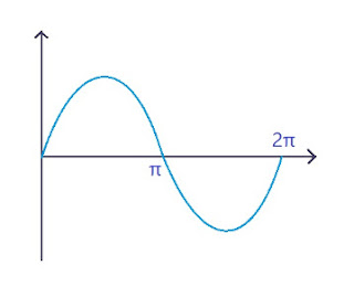
Instant Value = \(I_m \sin{\omega t}\)
For whole cycle the average value will be \(0\) as the area under the first cycle is \(0\). So, taking first half of the cycle from \(0 \rightarrow \pi\) \[ I_{avg} = \int_{0}^{\pi} \frac{I_m\sin{\omega t}}{\pi - 0} d\omega t \] (as average = sum of instant values / no. of instant values) \[ I_{avg} = \frac{I_m}{\pi} \int_{0}^{\pi} \sin{\omega t} d\omega t \] \[ I_{avg} = \frac{I_m}{\pi} [-\cos{\omega t}]_0^{\pi} \] \[ \boxed{I_{avg} = \frac{2I_m}{\pi} } \] \[ \boxed{I_{avg} = 0.637I_m } \]
Root Mean Square Values :
\[ i = I_m\sin{\omega t} \] Squaring both the sides \[ i^2 = I_m^2 \sin^2{\omega t} \] \[ i^2 = I_m^2 \left(\frac{1 - \cos{\omega t}}{2} \right) \] Taking average of given value : \[ i_{avg}^2 = \frac{I_{m}^2}{2} \int_{0}^{\pi} \frac{1 - \cos{2\omega t}}{\pi}d\omega t \] \[ i_{avg}^2 = \frac{I_m^2}{2\pi} \left[ [\omega t]^{\pi}_0 - \left[ \frac{\sin{2\omega t}}{2} \right]^{\pi}_0 \right] \] \[ i_{avg}^2 = \frac{I_m^2}{2\pi} \times \pi \] \[ i_{av}^2 = \frac{I_m^2}{2} \] On taking square root \[ \boxed{i_{rms} = \frac{I_m}{\sqrt{2}}} \] \[ \boxed{ i_{rms} = 0.707I_m } \] -
Form Factor & Peak Factor
Form Factor : Ratio of RMS value to the average value of altenating quantity \[ K_f = \frac{\text{RMS value}}{\text{Average value}} = \frac{E_{rms}}{E_{avg}} = \frac{\frac{E_m}{\sqrt{2}}}{\frac{2E_m}{\pi}} = 1.11 \]
Peak Factor : Ratio of Peak or Maximum value to RMS value of an alternating quantity \[ K_p = \frac{\text{Max. value}}{\text{RMS value}} = \frac{E_m}{\frac{E_m}{\sqrt{2}}} = 1.414 \] -
Active & Reactive components of Circuit Current
Active Component : \(I\cos{\phi} \longrightarrow\) the component which is in phase with the applied voltage \(V\) : also called as "Wattful component"
Reactive Component : \(I\sin{\phi} \longrightarrow \) the component which is out of phase with the applied voltage : also called as "Wattless component"
-
Power Factor & Quality Factor
Power Factor : a) Cosine of the phase angle between \(V\) and \(I\) i.e. \(\cos{\phi} \) b) Ratio of Resistance to Impedance \[ \cos{\phi} = \frac{R}{Z} \] c) Ratio of active power to apparent power \[ \cos{\phi} = \frac{\text{Active Power}}{\text{Apparent Power}} \] Note : P.F. cannot be greater than 1
Quality Factor : Reciprocal of Power factor is Quality Factor \[ \text{Q-factor } = \frac{1}{\cos{\phi}} = \frac{Z}{R} \] Also, \[ \text{Q-factor } = 2\pi \frac{\text{Max. Energy stored}}{\text{Energy dissipated per cycle}} \] -
Active, Reactive & Apparent Power
Apparent Power : the product of RMS values of applied voltage and circuit current \[ S = V_{rms}I_{rms} \] \[ \text{Unit : Volt-Ampere (VA) } \] Active Power : the product of apparent power and the power factor
it is due to the resistive part of the circuit \[ P = V_{rms}I_{rms}\cos{\phi} \] \[ \text{Unit : Watts (W)} \] Reactive Power : the product of apparent power and the sin of phase difference between \(V\) and \(I\)
also called as "Wattless Power" \[ Q = V_{rms}I_{rms}\sin{\phi} \] \[ \text{Unit : Volt-Ampere-Reactive (VAR) } \] -
AC Circuit containing purely Resistive load
Let us assume that a purely resistive load \(R \omega\) is connected across a supply of \( V = V_m\sin{\omega t} \longrightarrow (1) \)

\[ i = \frac{V}{R} \hspace{20pt} \text{[Ohm's law]} \] Putting value of \(V\) from (1) \[ i = \frac{V_m\sin{\omega t}}{R} \] \[ \boxed{i = I_m\sin{\omega t} } \longrightarrow (2) \] Comparing (1) and (2)
Voltage and Current are in same phase. Its phasor diagram is,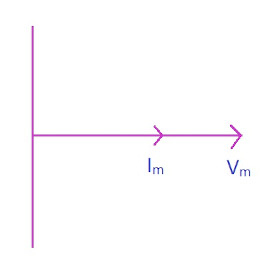
Power Dissipated : \[ P = Vi \] Putting values of \(V\) and \(i\) in \[ P = V_m\sin{\omega t} \times I_m\sin{\omega t} \] \[ P = V_mI_m\sin^2{\omega t} \] \[ P = V_mI_m \left( \frac{1 - \cos{2\omega t}}{2} \right) \] \[ P = \frac{V_mI_m}{2} - \frac{V_mI_m\cos{2\omega t}}{2} \] Neglecting the fluctuating part \[ P = \frac{V_mI_m}{2} \] \[ P = \frac{V_m}{\sqrt{2}} \frac{I_m}{\sqrt{2}} \] \[ \boxed{P = V_{rms}I_{rms}} \]
-
AC Circuit containing purely Inductive load
Let us assume that a purely inductive load to be connected in series across voltage supply of \(V = V_m\sin{\omega t} \longrightarrow (1)\)
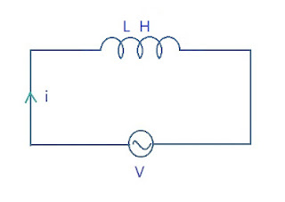
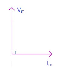
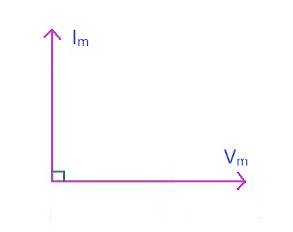
e.m.f. induced is given as: \[ v = L\frac{di}{dt} \] \[ V_m\sin{\omega t} = L\frac{di}{dt} \] \[ \int \frac{V_m\sin{\omega t}}{L}dt = \int di \] \[ i = \frac{V_m}{L} \int \sin{\omega t}dt \] \[ i = \frac{V_m}{L} \left( \frac{-\cos{\omega t}}{\omega} \right) \] \[ i = \frac{V_m}{\omega L} \sin{(\omega t - \pi /2)} \] Comparing it to Ohm's Law \[ \boxed{X_L = \omega L} \] \[ i = \frac{V_m}{X_L} \sin{(\omega t - \pi /2)} \] \[ \boxed{i = I_m\sin{(\omega t - \pi /2)}} \] For purely inductive load \(I\) lags behind \(V\) by \(90^\circ\). Its phasor diagram is,
Power : \[ P = VI \] \[ P = V_m\sin{\omega t}I_m\sin{(\omega t - \pi /2)} \] \[ P = -V_mI_m\sin{\omega t}\cos{\omega t} \] \[ P = -2 \times \frac{V_mI_m\sin{\omega t}\cos{\omega t} }{2} \] \[ P = \frac{-V_mI_m}{2}\sin{2\omega t} \] Neglecting the fluctuating part \[ \boxed{P = 0} \]
-
AC Circuit containing purely Capacitive load
Let us assume that a purely capacitive load of capacitance \(C\) \(F\) to be connected in series across voltage supply of \(V = V_m\sin{\omega t} \longrightarrow (1)\)

The charge stored by capacitor is given as \[ q = CV \] \[ i = \frac{dq}{dt} \] \[ i = C\frac{dV}{dt} \] \[ i = C\frac{d}{dt}V_m\sin{\omega t} \] \[ i = CV_m\omega \cos{\omega t} \] \[ i = \omega CV_m\sin{(\omega t + \pi /2)} \] Comparing with Ohm's Law \[ \boxed{X_C = \frac{1}{\omega C} = \frac{1}{2\pi fC} } \] \[ i = \frac{V_m}{X_C}\sin{(\omega t + \pi /2)} \] \[ \boxed{i = I_m\sin{(\omega t + \pi /2)}} \longrightarrow (2) \] For purely Capacitive load, current \(I\) leads \(V\) by \(90^\circ \). Its phasor diagram is,
Power : \[ P = Vi \] \[ P = V_m\sin{\omega t}I_m\sin{(\omega t + \pi /2)} \] \[ P = V_mI_m\sin{\omega t}\cos{\omega t} \] \[ P = 2 \times \frac{V_mI_m\sin{\omega t}\cos{\omega t}}{2} \] \[ P = \frac{V_mI_m}{2}\sin{2\omega t} \] Neglecting fluctuating part \[ \boxed{P = 0} \]
-
R-L Circuit
Consider a circuit consisting of resitor \(R\) and an inductive coil of inductance \(L\) connected in series. Since it includes inductor \(I\) will lag behind \(V\) by some phase difference \(\phi\) \[V = V_m\sin{\omega t}, i = I_m\sin{(\omega t - \phi)} \]

\[ V = \sqrt{V_L^2 + V_R^2} \] \[ V = \sqrt{(IR)^2 + (X_L)^2} \] \[ V = I\sqrt{R^2 + X_L^2} \] \[ V = IZ \] \[ \text{Impedance, } Z = \sqrt{R^2 + X_L^2} \] \[ \tan{\phi} = \frac{V_L}{V_R} = \frac{X_L}{R} \] \[ \boxed{ \phi = \tan^{-1}{\frac{X_L}{R}} } \] Power Factor : \[ \boxed{\cos{\phi} = \frac{R}{Z} } \] \[ \boxed{P = VI\cos{\phi}} \]
Sample Problem :
A \(4\Omega\) resitor is connected to \(10mH\) inductor across \(100V, 50Hz\) voltage source in series. Find
(a) Input current
(b) Voltage drop across inductor and resistor
(c) Power Factor
(d) Power consumedSolution :
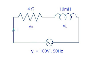
\[ R = 4\Omega, L - 10mH, X_L = \omega L = 2\pi fL \] \[ X_L = 2\pi \times 50 \times 10 \times 10^{-3} = 3.142\Omega \] \[ z = \sqrt{R_2 + X_L^2} \] \[ = \sqrt{4^2 + (3.142)^2} \] \[ = 5.086\Omega \] (a) Input Current : \[ I = \frac{V}{Z} = \frac{100}{5.086} = 19.66A \] (b) Voltage Drop across Resistor \[ I = 19.66A \] \[ V_R = IR = 19.66 \times 4 \] \[ V = 78.64V \] Voltage Drop across Inductor : \[ V_L = IX_L = 19.66 \times 3.142 \] \[ V_L = 61.77V \] (c) Power Factor \[ = \frac{R}{Z} = \frac{4}{5.086} = 0.786 \] (d) Power consumed = \[ VI\cos{\phi} = 100\times 19.66 \times 0.786 \] \[ = 1546W \]
-
R-C Circuit
Consider a circuit consisting of resitor \(R\) and a capacitor of capacitance \(C\) connected in series. Since it includes capacitor \(I\) leads \(V\) by some phase difference \(\phi\) [V = V_m\sin{\omega t}, i = I_m\sin{(\omega t + \phi)} \]

\[ V = \sqrt{V_C^2 + V_R^2} \] \[ V = \sqrt{(IR)^2 + (X_C)^2} \] \[ V = I\sqrt{R^2 + X_C^2} \] \[ V = IZ \] \[ \text{Impedance, } Z = \sqrt{R^2 + X_C^2} \] \[ \tan{\phi} = \frac{V_C}{V_R} = \frac{X_C}{R} = \frac{1}{\omega CR} \] \[ \boxed{ \phi = \tan^{-1}{\frac{X_C}{R}} } \] Power Factor : \[ \boxed{\cos{\phi} = \frac{R}{Z} } \] \[ \boxed{P = VI\cos{\phi}} \]
-
R-L-C Circuit

\[ V = IR, \] \[V_L = IX_L, \hspace{10pt} \text{ V leads I by }\pi /2 \] \[ V_C = IX_C, \hspace{10pt} \text{I leads V by }\pi /2 \] If \(V_L\) > \(V_C\), \[ V = \sqrt{(V_R)^2 + (V_L - V_C)^2} \] \[ V = \sqrt{IR^2 + (IX_L - IX_C)^2} \] \[ V = I \sqrt{R^2 + (X_L - X_C)^2} \] \[ \boxed{Z = \sqrt{ R^2 + (X_L - X_C)^2 }} \] If \(X_C > X_L\) or \(V_C > V_L\) \[ \boxed{Z = \sqrt{ R^2 + (X_C - X_L)^2 }} \] \[ \tan{\phi} = \frac{V_L - V_C}{V_R} \] \[ \boxed{\phi = tan^{-1}\frac{V_L - V_C}{V_R} = \tan^{-1}\frac{X_L - X_C}{R} } \] Power factor : \[ \cos{\phi} = \frac{R}{Z} \] \[ \cos{\phi} = \frac{R}{\sqrt{R^2 + (X_L - X_C)^2}} \] Power consumed, \[ \boxed{P = VI\cos{\phi}} \]
-
Three Phase AC Circuit
We study two types of connections in 3 phase systems: Star and Delta connection.
Star Connection
All the three terminals are connected to a common point. Also called as Y connection.

Line Currents : \(I_A = I_B = I_C = I_L \)
Line Voltages : \(V_{AB} = V_{AC} = V_{BC} = V_L \)
Phase Currents : \(I_{NA} = I_{NB} = I_{NC} = I_{P} \)
Phase Voltages : \(V_{A} = V_{B} = V_{C} = V_{P} \)
Relationship between Line and Phasor Currents
As we can see from the diagram \[ I_{NA} = I_A \] \[ I_{NC} = I_C \] \[ I_{NB} = I_B \] \[ \Rightarrow \boxed{I_P = I_L} \]
Relationship between Line and Phasor Voltages

\[ V_{AB} = V_A - V_B \] \[ = \sqrt{(V_A)^2 + (V_B)^2 + 2V_AV_B\cos{60^o}} \] \[ = \sqrt{V_A^2 + V_B^2 + V_AV_B} \] As \(V_A = V_B = V_C \) \[ V_{AB} = \sqrt{3V_A^2} = \sqrt{3}V_A \] \[ \Rightarrow \boxed{V_L = \sqrt{3}V_P} \] Power : Active Power in 1 phase = \(V_PI_P\cos{\phi}\)
Active Power in 3 phase, \[ P_T = 3V_PI_P\cos{\phi} \] \[ V_P = \frac{V_L}{\sqrt{3}}, I_P = I_L \] \[ P_T = 3\frac{V_L}{\sqrt{3}}I_L\cos{\phi} \] \[ \boxed{P_T = \sqrt{3}V_LI_L\cos{\phi} } \] Reactive Power : \[ Q_T = \sqrt{3}V_LI_L\sin{\phi} \] Apparent Power : \[ S_T = \sqrt{3}V_LI_L \]
Delta Connection
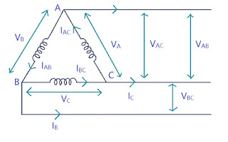
Line Currents : \(I_A = I_B = I_C = I_L \)
Line Voltages : \(V_{AB} = V_{AC} = V_{BC} = V_L \)
Phase Currents : \(I_{AB} = I_{AC} = I_{BC} = I_{P} \)
Phase Voltages : \(V_{A} = V_{B} = V_{C} = V_{P} \)
Relationship between Line and Phasor Voltages
As we can see from the diagram \[ V_{A} = V_{AC} \] \[ V_{B} = V_{AB} \] \[ V_{C} = V_{BC} \] \[ \Rightarrow \boxed{V_L = V_P} \]
Relationship between Line and Phasor Currents

\[ I_A = I_{AC} - I_{AB} \] \[ = I_{AC} + (-I_{AB}) \] \[ = \sqrt{I_{AC}^2 + I_{AB}^2 + 2I_{AC}I_{AB}\cos{60^o}} \] As \(I_{AC} = I_{AB} = I_{BC} \) \[ \Rightarrow I_A = \sqrt{3I_{AC}^2} = \sqrt{3}I_{AC} \] \[ \Rightarrow \boxed{I_L = \sqrt{3}I_P} \] Power : Active Power in 1 phase = \(V_PI_P\cos{\phi}\)
Active Power in 3 phase, \[ P_T = 3V_PI_P\cos{\phi} \] \[ I_P = \frac{I_L}{\sqrt{3}}, V_P = V_L \] \[ P_T = 3V_L\frac{I_L}{\sqrt{3}}\cos{\phi} \] \[ \boxed{P_T = \sqrt{3}V_LI_L\cos{\phi} } \] Reactive Power : \[ Q_T = \sqrt{3}V_LI_L\sin{\phi} \] Apparent Power : \[ S_T = \sqrt{3}V_LI_L \]


